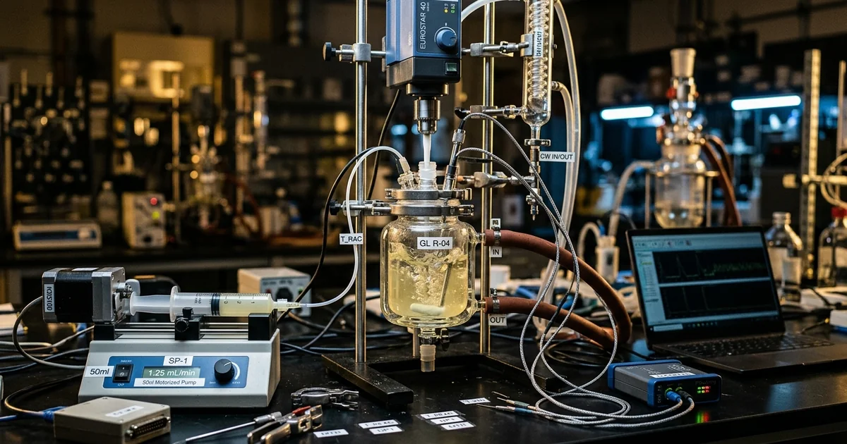
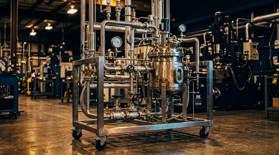
A hydrogenation that ran clean and selective in a 500 mL flask loses four points of yield the first time it runs in the 6 m³ plant reactor. Nobody can say why. The kinetics did not change. What changed is everything around the reaction — how fast the vessel mixes, how quickly it heats and cools, how long a molecule sits near a hot wall. A scale-down model is the discipline of building a laboratory experiment that reproduces the conditions the plant will impose. Bench data then predicts plant performance instead of flattering it. Get it right and the first commercial batch behaves like the last lab batch. Get it wrong and you find the gap after the capital is spent and the customer is waiting. This guide covers why lab and plant diverge, how to choose the variable a scale-down model must hold constant, how to design the study, and where these models break down. It reflects how we build the laboratory programme in our chemical reaction engineering practice before a process is transferred.
Why a Reaction That Works in the Lab Fails in the Plant
The reaction rate is set by chemistry and is scale-independent; the transport rates around it are not. As a vessel grows, its volume rises with the cube of linear size while its heat-transfer area rises only with the square. Every rate that depends on area per unit volume falls away. Mixing that was effectively instant in a flask now takes seconds or minutes in a stirred tank reactor. The reaction has not slowed, but it is now competing with much slower physics, and that competition is what shifts the result.
The specific mechanisms that diverge on scale-up are:
- Heat transfer — the heat-transfer area to volume ratio (A/V) falls roughly in proportion to 1/L as linear size L grows. A batch a flask held isothermal on the bench now depends on active cooling that may not match the exotherm. This is the same area-to-volume collapse that governs heat removal in ethoxylation reactors.
- Bulk mixing — blend time rises with scale at constant power per unit volume. A feed that dispersed instantly in the lab now forms a concentrated plume that sees a local stoichiometry far from the batch average.
- Micromixing — mixing down toward the Kolmogorov microscale and the molecular scale slows, so a fast reaction racing a by-product-forming one shifts toward the by-product. The Villermaux–Dushman and Bourne reactions are the standard test systems used to quantify this.
- Solids suspension and gas dispersion — the impeller speed that just suspended a catalyst in a flask can leave a settled layer in a tall vessel. The Zwietering correlation for just-suspended impeller speed describes that shift, and gas–liquid mass transfer per unit volume also drops.
- Residence time and its distribution — additions take longer and hold steps stretch. A real vessel mixes less completely than an ideal continuous stirred-tank reactor (CSTR) and less cleanly than an ideal plug flow reactor, so its residence time distribution smears the reaction history.
None of this means the lab lied. It means the lab ran a physically different experiment, one with faster heat removal and faster mixing than the plant can provide. A scale-down model makes the lab run the plant's experiment instead — and the first step is working out which of these mechanisms is the one that decides the outcome.
What a Scale-Down Model Actually Is
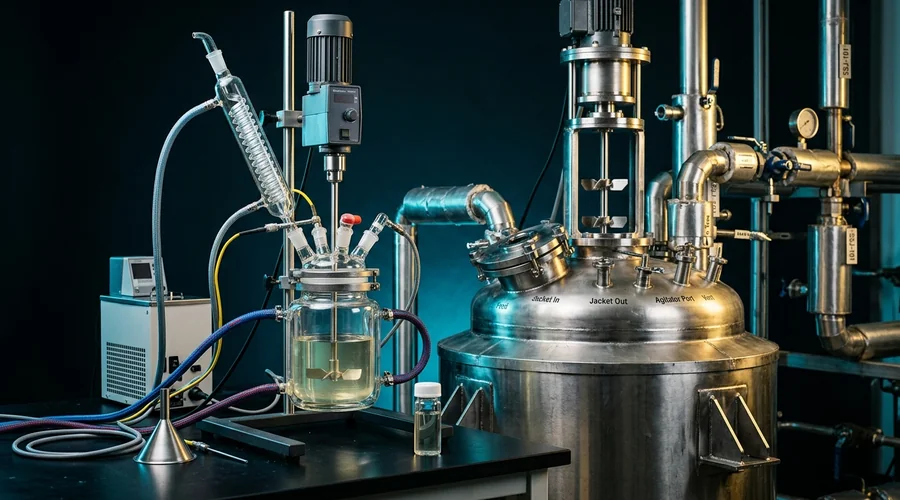
A scale-down model is a small-scale experiment deliberately constrained to match the plant on the rate-limiting phenomenon, while accepting a mismatch on everything else. It is the inverse of scale-up. Rather than asking how to make a process bigger, you ask what the large vessel does to the chemistry and then impose that on a one-litre reactor. The model is only ever as good as the identification of the limiting regime, so that identification is where the real work sits. Everything downstream is execution.
Building one follows a clear logic:
- Characterise the plant reactor — geometry, impeller type, installed cooling as an overall heat transfer coefficient (U) and area, feed points, and the achievable agitation range. Take this from the equipment data sheet and, where the vessel exists, from tracer and heat-transfer tests.
- Identify the controlling regime — decide whether the outcome is limited by heat removal, bulk mixing, micromixing, mass transfer, or genuine kinetics. A Damköhler number argument, comparing the reaction rate to the relevant transport rate, tells you which side dominates.
- Reproduce that regime at small scale — set the lab reactor so its limiting rate matches the plant's. That can mean running the stirrer slower or the addition faster than lab habit would suggest.
- Accept the compromises — the model will not match the plant on the phenomena that do not control the result, and it should not try to.
Once the regime is named, it dictates which variable you hold constant across the two scales. That choice is the subject of the next section, and it is the one most often made by default rather than on purpose.
The scale-down choice in one picture: hold the invariant the chemistry needs, and let the over-determined groups float.
Choosing the Controlling Variable: What to Hold Constant
You cannot hold every dimensionless group constant across scales at once. Geometric similarity plus equal impeller Reynolds number plus equal Froude number is over-determined, and something always has to give. Dimensional analysis through the Buckingham Pi theorem tells you which groups exist; the chemistry tells you which one to protect. That single choice decides what your model is precise about.
| Invariant held constant | Protects | Choose when limited by | What it sacrifices |
|---|---|---|---|
| Power per unit volume (P/V) | Turbulence intensity, heat-transfer coefficient, gas dispersion | Micromixing, gas–liquid mass transfer, heat removal | Blend time rises with scale; tip speed differs |
| Impeller tip speed (πND) | Maximum shear, drop and particle break-up | Crystal or droplet size, shear-sensitive polymer or biocatalyst | P/V falls sharply with scale |
| Blend time | Bulk homogeneity, feed distribution | Macromixing of a fast reaction fed into the batch | Needs impractically high P/V at large scale |
| Impeller Reynolds number | Flow-regime similarity | Laminar or transitional systems only | P/V and tip speed both diverge in turbulent tanks |
| Feed rate matched to cooling | Exotherm-to-cooling-capacity balance | Exothermic semi-batch reactions | Absolute batch time; needs measured plant U and area |
| Suspension margin (N/Njs) | Solids fully suspended, catalyst fully available | Slurry and solid-catalysed reactions | P/V, especially in tall vessels |
The common default for stirred-tank chemistry is constant P/V. It keeps both the small-scale turbulence and the jacket heat-transfer coefficient roughly constant, and most specialty reactions are limited by heat or by micromixing. But a shear-sensitive crystallisation scales on tip speed, and an exothermic semi-batch reaction scales on the feed rate the plant cooling can absorb. That is why the reactor configuration you are transferring into matters as much as the stirrer speed. For non-Newtonian systems the Metzner–Otto correlation links stirrer speed to an effective shear rate, and for slurries the Zwietering correlation sets the suspension baseline. Professional bodies such as the American Institute of Chemical Engineers and the Institution of Chemical Engineers publish the mixing and scale-up correlations these choices rest on.
Pick the wrong invariant and the scale-down model is exact about the wrong thing. It will reproduce a quantity the plant does not care about and drift on the one it does. With the invariant chosen, the lab study can be designed around it.
Designing the Laboratory Study
A scale-down model is a piece of equipment plus a protocol. The equipment has to let you vary the limiting rate on its own. The protocol has to probe the range the plant might actually see, not just its nominal set point. This is where reaction calorimetry and a structured design of experiments earn their cost, because they turn a handful of runs into a map rather than a set of anecdotes.
- Instrument the limiting phenomenon — if heat controls, run in a reaction calorimeter that measures heat-release rate against conversion, as covered in our guide to what reaction calorimetry measures and why scale-up needs it. If micromixing controls, use a bench reactor with a movable feed pipe and a variable-speed stirrer, characterised with a test reaction first.
- Bracket the plant, do not aim at its midpoint — run the scale-down model at the best and worst credible plant mixing, cooling and addition time. The plant's real operating point should sit inside your dataset, not at its edge.
- Vary one regime at a time — a structured design of experiments, in the spirit of Quality by Design and ICH Q8, separates a mixing effect from a temperature effect that a one-factor-at-a-time campaign confounds.
- Measure what fails at scale — impurity profile, particle size distribution, colour and residual starting material, not assay alone. Scale-up failures are usually about selectivity and quality rather than conversion.
- Log the trajectory, not just the endpoint — record temperature, pressure and addition profiles across the whole batch. The plant will only reproduce your result if it can reproduce your trajectory.
A well-designed scale-down study produces a response surface: outcome plotted against the controlling variable, across the range the plant can occupy. The plant then becomes a single point on that surface, one you can locate before the first batch runs. That is also most of the technical content a technology transfer package needs. The scale-down model is one of three tools, though, and knowing when it is enough saves the cost of the other two.
Scale-Down Model vs Pilot Plant vs Process Simulation
A scale-down model, a pilot plant and a process simulation answer overlapping questions at very different costs. The scale-down model is cheap and fast but depends on you having identified the right regime. The pilot plant tests the integrated process, including the transfers, holds and workup between reactions. The simulation extrapolates known physics but cannot invent kinetics or foresee fouling. Most technology transfers use two of the three, chosen by where the risk sits.
| Scale-down model | Pilot plant | Process simulation | |
|---|---|---|---|
| Cost and time | Low, weeks | High, months | Low to moderate, weeks |
| What it tests | One reactor step under plant-like transport | The whole train, including transfers, holds and workup | Mass and energy balance, equipment sizing, known unit operations |
| Main strength | Isolates the controlling phenomenon cheaply | Exposes interactions between steps and real materials of construction | Explores many cases fast; sizing and utilities |
| Main weakness | Only as good as the regime identification | Expensive, and still not full scale | No new kinetics, no fouling, no unexpected impurities |
| Best used for | Route and reactor selection, defining the operating window | De-risking the first commercial campaign, registration material | Feasibility, capital and operating cost estimates, debottlenecking |
The real question behind "do you always need a pilot plant" is whether the risk lies in the reactor or in the integration. A well-behaved single-step reaction with a clean scale-down model can sometimes go straight to the plant. A multi-step process with recycle, a solids-handling step, or an unfamiliar material of construction almost always earns its pilot campaign. Simulation sits alongside both. It is where geometric similarity and dimensional-analysis results get used to size equipment once the chemistry is pinned down. The three tools are complementary, and the scale-down model often tells you how much of the other two you need.
Where Scale-Down Models Break Down
A scale-down model fails in a few recognisable ways, and every one traces back to a phenomenon the scale-down model did not reproduce. When plant data misses the scale-down model, the useful question is not whether the model was wrong but which regime it left out. The direction and size of the miss usually point straight at the answer.
- Assay matches but impurities do not — micromixing was not reproduced, so the plant's slower molecular-scale mixing lets a fast side reaction proceed. Consequence: off-spec purity, a downgrade, or a rejected registration batch.
- Plant yield is lower and the batch runs longer — the heat-limited feed rate was faster in the lab than the plant cooling allows, so the plant slows the addition and holds longer at temperature. Consequence: campaign throughput below plan.
- An impurity appears only at plant scale — a hot-wall or long-residence pathway that the small vessel's high A/V and short hold times suppressed. Consequence: a new impurity to qualify, occasionally a genotoxic one needing tight control.
- The catalyst underperforms at scale — solids that were fully suspended in the lab settle partly in a tall plant vessel, so the effective loading is lower. The recovery and consistency trade-offs here are the ones set out in our guide to homogeneous versus heterogeneous catalysis. Consequence: incomplete conversion and longer batches.
- The model cannot be reconciled at all — usually two regimes changed at once and a one-factor design confounded them. The fix is a small structured re-study, not more plant batches.
The pattern is consistent: scale-down models fail on the phenomenon that was assumed not to matter. That is exactly why the regime-identification step deserves more scrutiny than the experimental work that follows it. A scale-down model that misses the plant is still worth having, because it tells you where to look.
A Framework for Building a Scale-Down Model
Building a scale-down model is a sequence, and working it in order means the questions that eliminate approaches are settled before the ones that only refine them. The output of the sequence is also most of what a technology transfer package needs, so none of the analysis is wasted.
- Define what success at scale means — the exact assay, impurity, particle size and colour targets the plant batch must hit. This decides what the scale-down model measures.
- Characterise the plant reactor — geometry, impeller, installed U and area, agitation range and feed points, from the data sheet and from tracer and heat-transfer tests where the vessel exists.
- Identify the controlling regime — heat, macromixing, micromixing, mass transfer or kinetics, using a Damköhler-type comparison of reaction rate to transport rate.
- Choose the invariant — P/V, tip speed, blend time, feed rate matched to cooling, or suspension margin, following directly from step 3.
- Build and characterise the lab reactor — instrument the limiting phenomenon and verify it with a test reaction or a calorimetric run before committing to the campaign.
- Run a bracketing design of experiments — best and worst credible plant conditions, one regime varied at a time, the full batch trajectory logged.
- Decide on the pilot — if the reactor risk is now low and the integration risk is low, transfer; otherwise pilot only the parts that stay uncertain.
Most processes that transfer cleanly had this work done before the first plant batch, not after it. The value is not in any single experiment but in knowing which experiment decides the outcome. That is what separates a technology transfer package that holds from one that generates a corrective-action list. If you are taking a process from bench toward production, our scale-up and process development service covers scale-down model design and the reaction engineering behind it. The wider route is set out in our guide to going from lab to market. Manufacturers building specialty chemical capacity in India and the wider Gulf increasingly commission this modelling work up front. A failed first campaign at a new site costs far more than the study that would have predicted it.
Frequently Asked Questions
What is a scale-down model?
A scale-down model is a small-scale experiment built to reproduce the conditions a production reactor imposes on a reaction. Bench data then predicts plant performance rather than flattering it. It is the inverse of scale-up. Instead of asking how to make a process bigger, you ask what the large vessel does to the chemistry, then impose that on a one-litre reactor.
The model is constrained to match the plant on whichever phenomenon controls the result, such as heat removal or micromixing, and it accepts a mismatch on everything else. Its value depends entirely on correctly identifying that controlling phenomenon before the experiments begin.
Why does a reaction work in the lab but fail in the plant?
The reaction rate is set by chemistry and does not change with scale, but every transport rate around it does. As a vessel grows, volume rises with the cube of linear size but heat-transfer area only with the square. The area available to remove heat per unit of batch falls. Mixing that was effectively instant in a flask now takes seconds or minutes, so a feed forms a concentrated plume and fast side reactions gain ground.
Solids that stayed suspended in the lab can settle in a tall plant vessel. The lab did not lie; it ran a physically different experiment, and a scale-down model exists to close that gap.
Which variable should you hold constant when scaling down?
You cannot hold every dimensionless group constant at once, so you protect the one the chemistry is most sensitive to. Constant power per unit volume is the common default for stirred-tank reactions because it keeps turbulence intensity and the heat-transfer coefficient roughly constant, which suits micromixing-limited and heat-limited systems.
Constant impeller tip speed is chosen for shear-sensitive systems such as crystallisations, droplet dispersions or biocatalysts. An exothermic semi-batch reaction is scaled on the feed rate the plant cooling can absorb, and a slurry reaction on the margin above the just-suspended impeller speed. The controlling regime dictates the invariant, not lab habit.
What is the difference between scale-up and scale-down?
Scale-up takes a working small-scale process and engineers a larger version of it, sizing equipment and setting operating conditions for the target output. Scale-down works in the opposite direction. It takes a known or planned plant reactor and recreates its limiting behaviour in a laboratory vessel, so development work runs under realistic constraints from the start.
Scale-up is a design activity; scale-down is a diagnostic and de-risking activity. Teams that only scale up often discover the transport limits of the plant after the capital is committed, whereas a scale-down model surfaces them while changes are still cheap.
Do you always need a pilot plant?
Not always. A single-step reaction that is well understood, with a clean scale-down model, can sometimes move straight to the plant. That is most defensible when the reactor is a known asset with measured heat-transfer and mixing data. A pilot plant earns its cost when the risk lies in the integration rather than in one reactor. Typical cases are multi-step sequences with recycle, solids handling, new materials of construction, or a workup that has never run at intermediate scale.
The scale-down model is often what tells you which case you are in, because it isolates the reactor risk and leaves the integration risk visible.
How accurate is a scale-down model?
A scale-down model is accurate on the phenomenon it was built to reproduce and unreliable on the phenomena it deliberately mismatches. If heat removal controls the outcome and the model matches the plant on the exotherm-to-cooling balance, it will predict yield and impurity trends well.
If micromixing also matters and was not reproduced, the model can match assay while missing an impurity by a wide margin. The useful discipline is to state in advance what the model is expected to predict and what it is not. A later mismatch then points straight at the regime that was left out.
Can you scale down a continuous process?
Yes, and it is often easier than scaling down a batch process. Continuous reactors are usually scaled by running longer or by adding parallel channels, not by enlarging a vessel. A bench continuous reactor can hold the same residence time, temperature profile and mixing intensity as the intended plant unit. The residence time distribution and the reaction environment then transfer directly.
The main scale-down questions for continuous systems are heat removal in larger tubes or plates, flow distribution across parallel paths, and fouling. A very small rig does not always reveal them. Even so, the gap between a well-designed continuous bench unit and its plant version is typically narrower than for batch.
Taking a Process From Bench to Plant?
Global Formulation provides route selection, scale-down model design and scale-up partnership for reactor-based processes — identifying the controlling regime, building the laboratory model that predicts your plant, and turning it into a technology transfer package that holds on the first campaign.
Talk to Our Process Team